2 Hours
Rmarkdown, and the knitr packagePlease share the following:
Automation or transformation: has the research paper changed much in the last 350 years (or why static PDFs are an underwhelming use of today’s technology)
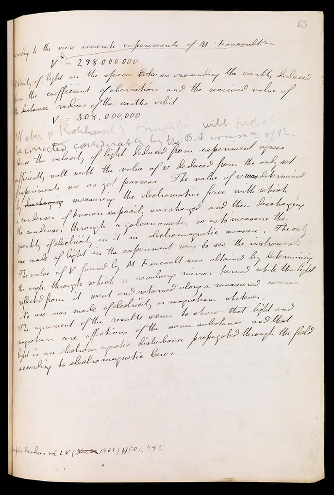
Original manuscript of James Clerk Maxwell’s paper on ‘A dynamical theory of the electromagnetic field’ published in the oldest scientific journal, Philosophical Transactions, in 1685. According to the publisher, the Royal Society:
The final sentence on this page records his crucial revelation regarding the nature of light: ‘The agreement of the results seems to show that light and magnetism are affections of the same substance and that light is an electromagnetic disturbance propagated through the field according to electromagnetic laws.’ (source: https://www.theguardian.com/higher-education-network/gallery/2015/feb/12/philosophical-transactions-of-the-royal-society-350-years-of-science-publishing-in-pictures)
Photograph: Royal Society’s collections
Source: Rallison, S.P., ‘What are Journals For?’, Ann R Coll Surg Engl. 2015 Mar; 97(2): 89-91. DOI: 10.1308/003588414X14055925061397
Now we’ll show you the final result (on our machine).
The first step in getting this dynmaic document is installing some software!
R is a programming language that is especially powerful for data exploration, visualization, and statistical analysis. To interact with R, we use RStudio. For this workshop you’ll need to install both R (version 3.4.3 or newer) and RStudio on your computer.
Install R by downloading and running this .exe file from CRAN. Also, please install the RStudio IDE. Note that if you have separate user and admin accounts, you should run the installers as administrator (right-click on .exe file and select “Run as administrator” instead of double-clicking). Otherwise problems may occur later, for example when installing R packages.
Install R by downloading and running this .pkg file from CRAN. Also, please install the RStudio IDE.
You can download the binary files for your distribution from CRAN. Or you can use your package manager (e.g. for Debian/Ubuntu run sudo apt-get install r-base and for Fedora run sudo dnf install R). Also, please install the RStudio IDE.
You also need to download some files for this workshop:
FSCI-2018-files.Now open Rstudio (Applications/Rstudio). Rstudio is the development environment where we’ll be working on our document. The main panel you’ll see on the left is the Console, where you can run R code. On the right is two panels - the upper contains your environment (what R can access), and the lower contains the files on your computer.
The first thing to do is install some packages. RStudio makes it easy to install new packages to do things you want. You can find packages by going to the ‘Packages’ tab in the lower right panel. You can install new packages by clicking the Install button and typing in the package name. For this workshop we’ll need the following packages:
tidyverseDTrorcidhttpuvNow let’s actually work with a document. Click in the Files tab in the lower
right panel. The file view in RStudio is just like
navigating in finder or windows explorer. Let’s find the FSCI-2018-files
folder we downloaded above. Go to Desktop and FSCI-2018-files. You’ll see
lots of files we’ll use during the workshop. Double click on
Base_2013_day1_in.Rmd.
You’ll see the document open in a new panel on the left hand side of the screen. This is an editor window, and you can change things in the document here. For now, just change the name in the document to your name.
Knitting is a process in Rstudio that takes a text document and turns it into an output (like html, docx, or html slides). Now click the knit button in the upper left hand corner of the editor. The first time you do this you’ll get a message that you need to install some packages. You’ll want to click Yes and wait for the packages to install. Once the installation you’ll see an interactive demonstration document!
You can output this single file in multiple formats. By default we’ve been generating .html files, but we can also output to a word document. If you click on the downward arrow next to the knit button we see some default formats. Click on Word, and a word document will appear.
While pdf is an option, this requires a TeX distribution which is complex to install and beyond the scope of this course.
You can also select other output forms that aren’t listed in the knitr
dropdown. Take a look at the document. You’ll see in the top a section called
output with sections under it like html_document. If we change the top
output knit will produce a different result. Try replacing word_document
with slidy_presentation. This is a html presentation that you can use in
any web browser.
Tomorrow we’ll start working with an actual research report !
Next: Basic Markdown